drumplot cookbook

In this example you will learn how to create a waveform object by loading a SAC file, extract 1 hour of data from that waveform object, and make a helical drum recorder plot using the drumplot class.

Another feature of drumplot is that it allows detected events, from a Catalog object, to be superimposed on the helicorder plot. In the example below this Catalog is generated by running an STA/LTA detection algorithm on the extracted 1-hour waveform object.

Contents

Load 1 day of data for REF.EHZ on 2009.03.22

% here we can either use scnlobject or ChannelTag to describe the
% net-sta-loc-chan we want. waveform understands both.
ctag = ChannelTag('AV.REF.-.EHZ')

% starttime in MATLAB datenum format
snum = datenum(2009,3,22);

% endtime (1 day after start)
enum=snum+1;

% create the datasource object - in this case it is a SAC file
ds = datasource('sac', 'SACDATA/REF.EHZ.2009-03-22T00:00:00.000000Z.sac');

% create the waveform object with this datasource, ChannelTag, starttime
% and endtime
w=waveform(ds, ctag, snum, enum);

ctag = 

<a href="matlab:help ChannelTag">ChannelTag</a> with network.station.location.channel:
   network: 'AV'
   station: 'REF'
  location: '-'
   channel: 'EHZ'

fill gaps, detrend, band pass filter

% in case there are gaps in the time series (marked by NaN) we can interpolate a
% meaningful value
w = fillgaps(w, 'interp');

% detrend the time series - this removes linear drift
w = detrend(w);

% create a Butterworth bandpass filter from 0.5 to 15 Hz, 2 poles
fobj = filterobject('b', [0.5 15], 2);

% apply the filter in both directions (acausal) - this is a zero phase
% filter which is helpful because it doesn't disperse different frequency
% components. the caveat is that it can spread energy so arrivals may appear
% slighter earlier than they actually are
w = filtfilt(fobj, w);

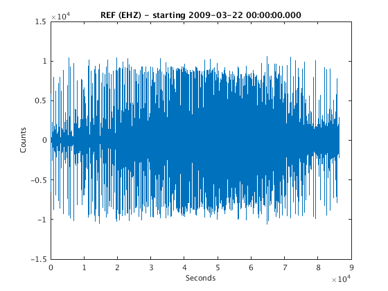
plot the waveform object

figure
plot(w)

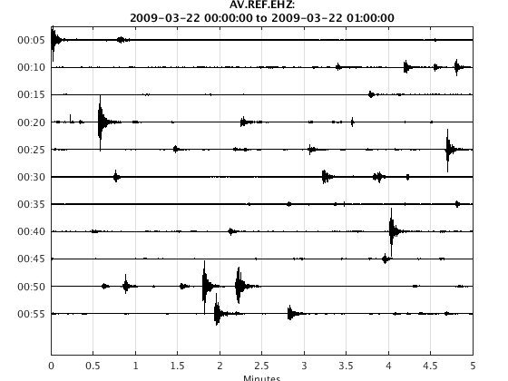
extract the first 1 hour of data and plot with 5 minutes per line

starttime = get(w,'start');
w2=extract(w, 'time', starttime, starttime + 1/24 )

% make a drumplot object. mpl means minutes per line and is set here to 5.
h2 = drumplot(w2, 'mpl', 5);

% plot the drumplot object - many events are visible, this is an earthquake
% swarm
plot(h2)

 
w2 =
 
 ChannelTag: AV.REF..EHZ       [network.station.location.channel]
      start: 2009-03-22 00:00:00.000
             duration(01:00:00.000)
       data: 360000 samples
       freq: 100.0000   Hz
      units: Counts
    history: [3 items], last modification: 22-Mar-2017 14:13:28
    With misc fields...
    * SCALE: 1
    * NZYEAR: 2009
    * NZJDAY: 81
    * NZHOUR: 0
    * NZMIN: 0
    * NZSEC: 0
    * NZMSEC: 0
    * IFTYPE: 1
    * IZTYPE: 9
    * LPSPOL: 0
    * LOVROK: 1
    * LCALDA: 1
    * KEVNM: -12345  -12345

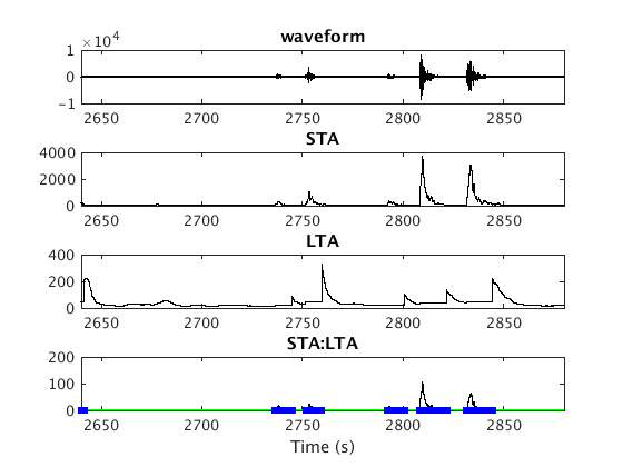
Run an STA/LTA detector on the waveform object to detect events

Compute STA/LTA ratio. In this example, trigger "ON" when STA/LTA exceeds 3, trigger "OFF" when this drops back below 1.5. If the trigger was on for at least 2 seconds, declare it as an event. All the events get saved into a Catalog object.

% set the STA/LTA detector
sta_seconds = 0.7; % STA time window 0.7 seconds
lta_seconds = 7.0; % LTA time window 7 seconds
thresh_on = 3; % Event triggers "ON" with STA/LTA ratio exceeds 3
thresh_off = 1.5; % Event triggers "OFF" when STA/LTA ratio drops below 1.5
minimum_event_duration_seconds = 2.0; % Trigger must be on at least 2 secs
pre_trigger_seconds = 0; % Do not pad before trigger
post_trigger_seconds = 0; % Do not pad after trigger
event_detection_params = [sta_seconds lta_seconds thresh_on thresh_off ...
    minimum_event_duration_seconds];

% run the STA/LTA detector. lta_mode = 'frozen' means the LTA stops
% updating when trigger is "ON".
[cobj,sta,lta,sta_to_lta] = Detection.sta_lta(w2, 'edp', event_detection_params, ...
    'lta_mode', 'frozen');

% not sure what this is for
set(gca, 'XLim', [44*60 48*60])

Event 1: 22-Mar-2009 00:00:47 to 22-Mar-2009 00:00:58
Event 2: 22-Mar-2009 00:07:05 to 22-Mar-2009 00:07:08
Event 3: 22-Mar-2009 00:08:06 to 22-Mar-2009 00:08:08
Event 4: 22-Mar-2009 00:08:23 to 22-Mar-2009 00:08:28
Event 5: 22-Mar-2009 00:09:11 to 22-Mar-2009 00:09:23
Event 6: 22-Mar-2009 00:09:32 to 22-Mar-2009 00:09:38
Event 7: 22-Mar-2009 00:09:47 to 22-Mar-2009 00:09:57
Event 8: 22-Mar-2009 00:13:46 to 22-Mar-2009 00:13:51
Event 9: 22-Mar-2009 00:15:34 to 22-Mar-2009 00:15:44
Event 10: 22-Mar-2009 00:17:15 to 22-Mar-2009 00:17:24
Got 46 events

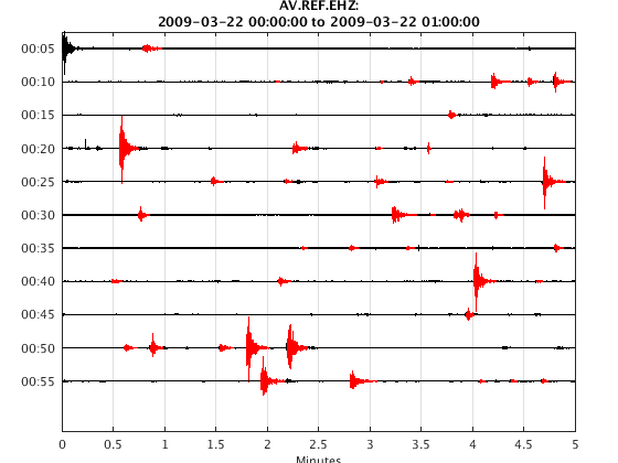
Plot detected events on top of the continuous drumplot

h3 = drumplot(w2, 'mpl', 5, 'catalog', cobj);
plot(h3)

Adding waveforms for each event in Catalog
..............................................
(Complete)

Published with MATLAB® R2015a