How to compute RSAM data
Contents
1. Introduction
Computing rsam data from waveform objects is easy to do with the waveform2rsam method. But waveform objects are generally no more than 1 hour long. So what if you want to compute RSAM data for days, weeks or months of waveform data? How do we set this up?
This is where we use "IceWeb", an application originally written in 1998 to process continuous waveform data into a variety of products for volcano observatory web pages, to aid rapid recognition of anomalous activity. Since we only want RSAM data in this case, we will drive this using iceweb.rsam_wrapper. To get help on this, use:
help iceweb.rsam_wrapper
RSAM data will be saved to binary "BOB" files in a directory "iceweb/rsam_data". So the final step in the tutorial will show how to load and plot these data.
The following is a fully worked example using the Sakurajima dataset for illustration.
2. Setup for the Redoubt 2009 example
Define datasource - where to get waveform data from
dbpath = fullfile(TESTDATA, 'css3.0', 'demodb')
datasourceObject = datasource('antelope', dbpath)
dbpath =

/home/t/thompsong/src/GISMO.website/testdata/css3.0/demodb


datasourceObject =

      type: ANTELOPE
  location: /home/t/thompsong/src/GISMO.website/testdata/css3.0/demodb
Define the list of channels to get waveform data for
ChannelTagList = ChannelTag.array('AV',{'REF';'RSO'},'','EHZ')
ChannelTagList =

<a href="matlab:help ChannelTag">ChannelTag</a> array (network.station.location.channel):
  AV.REF..EHZ
  AV.RSO..EHZ
Set the start and end times
startTime = datenum(2009,3,20,2,0,0)
endTime = datenum(2009,3,23,12,0,0)
startTime =

   7.3385e+05


endTime =

   7.3386e+05
We can't process more than 1 day of waveform data at a time, so we have to 'gulp it down' in non-overlapping timewindows of size 'gulpMinutes'. Experiments suggest 60 minutes is ideal, minimum 10 minutes, maximum 120 minutes.
gulpMinutes = 60;
RSAM data is traditionally computed with a sampling interval of 60 sec, with each RSAM value being the mean absolute value of the waveform data in a 60 sec window starting at that time. But with GISMO's implementation of RSAM, we can compute multiple RSAM datasets from the same waveform data, using different statistical measures and sampling intervals. We will compute: 1. traditional rsam: mean absolute value of 60-sec time windows 2. max absolute values of 10-sec time windows - great for highlighting events 3. median absolute values of 600-sec time windows - great for highlighting tremor
measures = {'mean';'max';'median'};
samplingIntervalSeconds = [60 10 600];
3. Call the rsam_wrapper
iceweb.rsam_wrapper('Redoubt', datasourceObject, ChannelTagList, ...
            startTime, endTime, gulpMinutes, ...
            samplingIntervalSeconds, measures);
2009/03/20 02 03 04 05 06 07 08 09 10 11 12 13 14 15 16 17 18 19 20 21 22 23
2009/03/21 00 01 02 03 04 05 06 07 08 09 10 11 12 13 14 15 16 17 18 19 20 21 22 23
2009/03/22 00 01 02 03 04 05 06 07 08 09 10 11 12 13 14 15 16 17 18 19 20 21 22 23
2009/03/23 00 01 02 03 04 05 06 07 08 09 10 11 COMPLETED
Note: this may take a long time to run, e.g. 1 week of data for 1 channel might take about 10 minutes on a desktop computer, reading data from a network-mounted drive.
4. Load RSAM data
The RSAM data computed have been stored in binary BOB files. To load these we use can loop through our channels, loading one file per channel, creating an array of RSAM objects.
Loading a single RSAM file is trivial. Here is the path to one of our files that iceweb.rsam_wrapper just created:
rsamfile = fullfile('iceweb', 'rsam_data', 'REF.EHZ.2009.mean.bob')
rsamfile =

iceweb/rsam_data/REF.EHZ.2009.mean.bob
To load this we use the 'read_bob_file' method:
s = rsam.read_bob_file(rsamfile)
Looking for file: iceweb/rsam_data/REF.EHZ.2009.mean.bob - found
Loading data from iceweb/rsam_data/REF.EHZ.2009.mean.bob, position 0 to 5.256000e+05 of 525600
mean of data loaded is 1.030975e+33

s =

  rsam with properties:

                 dnum: [1x525600 double]
                 data: [1x525600 double]
              measure: ''
      seismogram_type: ''
                units: ''
                files: [1x1 struct]
           ChannelTag: [1x1 ChannelTag]
              request: [1x1 struct]
                 snum: 733774
                 enum: 7.3414e+05
                  sta: {''}
                 chan: {''}
    sampling_interval: 60.0000
                stats: [1x1 struct]
But in a more general way, we can load multiple RSAM files using a filepattern. In a filepattern SSSS is a placeholder for station, CCC is a placeholder for channel, YYYY for year, and MMMM for measure. IceWeb creates RSAM files using the 'SSSS.CCC.YYYY.MMMM.bob' filepattern.
If you don't want to load all data from all the files matching that pattern, you can also specify an optional start time (snum) and end time (enum).
s = [];
for c=1:numel(ChannelTagList)
    sta = ChannelTagList(c).station();
    chan = ChannelTagList(c).channel();
    filepattern = fullfile('iceweb', 'rsam_data', 'SSSS.CCC.YYYY.MMMM.bob')
    r = rsam.read_bob_file(filepattern, 'sta', sta, 'chan', chan, ...
        'snum', startTime, 'enum', endTime, 'measure', 'mean');
    s = [s r];
end
s
filepattern =

iceweb/rsam_data/SSSS.CCC.YYYY.MMMM.bob

Looking for file: iceweb/rsam_data/REF.EHZ.2009.mean.bob - found
Loading data from iceweb/rsam_data/REF.EHZ.2009.mean.bob, position 112441 to 117360 of 525600
mean of data loaded is 2.451454e+02

filepattern =

iceweb/rsam_data/SSSS.CCC.YYYY.MMMM.bob

Looking for file: iceweb/rsam_data/RSO.EHZ.2009.mean.bob - found
Loading data from iceweb/rsam_data/RSO.EHZ.2009.mean.bob, position 112441 to 117360 of 525600
mean of data loaded is 2.160985e+02

s =

  1x2 rsam array with properties:

    dnum
    data
    measure
    seismogram_type
    units
    files
    ChannelTag
    request
    snum
    enum
    sta
    chan
    sampling_interval
    stats
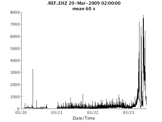
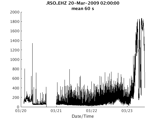
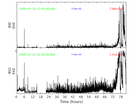
5. Plotting RSAM data
There are two ways to plot RSAM data. The first is to use the plot method, which generates one figure per channel:
plot(s);
The second is plot_panels, which generates one subplot per channel:
plot_panels(s)
This is the end of this tutorial.